Algebra 1 Scatter Plots, Lines of Fit and Two-Way Tables Worksheet Solutions (PDF)

This algebra 1 scatter plots answers for Algebra 1 covers scatter plots, lines of fit and two-way tables (Common Core S-ID.B.5, S-ID.B.6, S-ID.C.7, S-ID.C.8, S-ID.C.9), with a free PDF to print.
Algebra 1 · Common Core State Standards: S-ID.B.5, S-ID.B.6, S-ID.C.7, S-ID.C.8, S-ID.C.9
Algebra 1 scatter plots answers: exercises 1 to 10
Exercise 1 – Positive association
As \(x\) increases, \(y\) increases.
Positive association
Exercise 2 – Negative association
As \(x\) increases, \(y\) decreases.
Negative association
Exercise 3 – No association
There is no pattern: \(y\) does not change in a predictable way as \(x\) changes.
No association
Exercise 4 – Equation of a line of fit
Slope: \(\frac{34 – 10}{8 – 2} = 4\). Then \(10 = 4(2) + b\), so \(b = 2\).
\(y = 4x + 2\). At \(x = 5\): \(4(5) + 2 = 22\).
\(y = 4x + 2\); 22
Exercise 5 – Interpret the slope and intercept
The slope 2.5: each additional hour studied is associated with a 2.5-point increase in the predicted score.
The y-intercept 40: the predicted score for a student who studies 0 hours.
2.5 points per hour; 40 points at 0 hours
Exercise 6 – Predict from the line
\(y = -3(7) + 50 = 29\).
Solve \(-3x + 50 = 17\): \(-3x = -33\), so \(x = 11\).
29; 11
Exercise 7 – Compute a residual
Residual = actual – predicted = \(31 – 28.4 = 2.6\).
The point is above the line.
2.6
Exercise 8 – Residual from an equation
Predicted: \(1.5(6) + 4 = 13\). Residual: \(11 – 13 = -2\).
The point is below the line.
Predicted 13; residual -2
Exercise 9 – Residuals for three points
Predicted values: \(4, 6, 8\).
Residuals (actual – predicted): \(5 – 4 = 1\), \(6 – 6 = 0\), \(10 – 8 = 2\).
1, 0, 2
Exercise 10 – Interpret correlation
(a) Close to 1: a strong positive linear relationship. (b) Negative but closer to 0 than to -1: a weak negative relationship. (c) Near 0: essentially no linear relationship.
strong positive; weak negative; no linear relationship
Exercises 11 and up
Exercise 11 – Correlation and causation
No. Both increase when the weather is hot and sunny. Hot weather is a lurking variable that explains the association.
No; the weather is a lurking variable
Exercise 12 – Interpolation and extrapolation
At \(x = 25\), inside the data range (interpolation): \(0.8(25) + 12 = 32\). This is reasonable.
At \(x = 100\), far outside the range (extrapolation): the trend may not continue.
x = 25 is reasonable (32); x = 100 is unreliable
Exercise 13 – Complete a two-way table
Row totals: \(30 + 20 = 50\) and \(10 + 40 = 50\). Column totals: \(30 + 10 = 40\) and \(20 + 40 = 60\). Grand total: \(50 + 50 = 100\).
Totals 50, 50, 40, 60; grand total 100
Exercise 14 – Joint and marginal frequencies
Joint: \(\frac{40}{100} = 40\%\).
Marginal for walkers: \(\frac{40}{100} = 40\%\).
40% and 40%
Exercise 15 – Conditional frequency
Grade 7 students who walk: \(\frac{30}{50} = 60\%\).
Walkers in grade 7: \(\frac{30}{40} = 75\%\).
60%; 75%
Exercise 16 – Least-squares line
Predict: \(6.4(4.5) + 45.4 = 28.8 + 45.4 = 74.2\).
Since \(r \approx 0.999\) is very close to 1, the linear relationship is very strong and positive.
About 74.2 points; very strong positive
Exercise 17 – Line of fit in context
Slope: \( rac{75 – 35}{30 – 10} = 2\). Then \(35 = 2(10) + b\), so \(b = 15\).
\(y = 2x + 15\). The seedling grows about 2 cm per day. At day 20: \(2(20) + 15 = 55\) cm.
\(y = 2x + 15\); 2 cm per day; 55 cm
Exercise 18 – Used car values
Slope \(-1500\): the car loses about $1,500 in value each year. Intercept 22,000: the value when new.
At 4 years: \(-1500(4) + 22000 = 16000\). For $10,000: \(-1500x + 22000 = 10000\), so \(x = 8\).
$1,500 per year; $22,000 new; $16,000; 8 years
Exercise 19 – Residual plot
A residual plot with no pattern supports a linear model. A U-shaped pattern means the points curve away from the line (positive, then negative, then positive residuals).
No; a curved model would fit better
Exercise 20 – Breakfast and scores
No. The study shows association, not causation. Families with more time, sleep, or resources may both serve breakfast and support learning.
No; for example, sleep or family resources
Key facts behind this algebra 1 scatter plots answers
- A scatter plot can show positive, negative, or no association.
- In a line of best fit, the slope is the rate of change and the intercept is the predicted value at x = 0.
- Residual = actual value – predicted value.
- The correlation coefficient r is between -1 and 1; correlation does not imply causation.
- Two-way tables give joint, marginal, and conditional relative frequencies.
How to use this algebra 1 scatter plots answers
Cover each solution, solve the exercise again, then uncover it and compare every line. If your answer differs, find the first step that changed and redo the exercise from there.
Download the algebra 1 scatter plots answers as a PDF with the button below and keep it with your notes.
Download the algebra 1 scatter plots answers as a PDF with the button below and keep it with your notes.
All Algebra 1 chapters: Algebra 1 math.
Free printable PDF
Algebra 1 Scatter Plots, Lines of Fit and Two-Way Tables Worksheet Solutions
Download PDF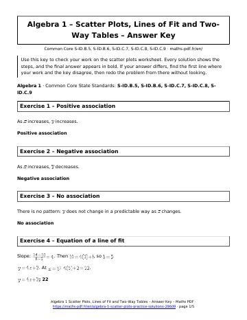
More Algebra 1 math
Lessons
See all





Worksheets
See all





Tests
See all Writing Linear Equations and Functions Test with Point Values
- Solving Quadratic Equations Test with Point Values
- Graphing Quadratic Functions and Transformations Test with Point Values
- Slope and Rate of Change Test with Point Values
- Solving Linear Equations in One Variable Test with Point Values
- Graphing Linear Equations Test with Point Values