
Algebra 1 Scatter Plots, Lines of Fit and Two-Way Tables Worksheet (PDF)

This algebra 1 scatter plots worksheet for Algebra 1 covers scatter plots, lines of fit and two-way tables (Common Core S-ID.B.5, S-ID.B.6, S-ID.C.7, S-ID.C.8, S-ID.C.9), with a free PDF to print.
Algebra 1 · Common Core State Standards: S-ID.B.5, S-ID.B.6, S-ID.C.7, S-ID.C.8, S-ID.C.9
Algebra 1 scatter plots worksheet: exercises 1 to 10
Exercise 1 – Positive association
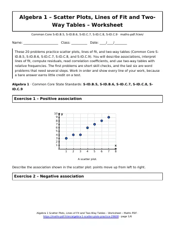
Describe the association shown in the scatter plot: points move up from left to right.
Exercise 2 – Negative association
Describe the association shown in the scatter plot: points move down from left to right.
Exercise 3 – No association
Describe the association shown in the scatter plot: points are scattered with no clear direction.
Exercise 4 – Equation of a line of fit
Exercise 5 – Interpret the slope and intercept
Exercise 6 – Predict from the line
Exercise 7 – Compute a residual
Exercise 8 – Residual from an equation
Exercise 9 – Residuals for three points
The line of fit is \(y = 2x + 2\). Find the residuals for the data points \((1, 5), (2, 6), (3, 10)\).
Exercise 10 – Interpret correlation
Exercises 11 and up
Exercise 11 – Correlation and causation
Exercise 12 – Interpolation and extrapolation
Exercise 13 – Complete a two-way table
Fill in the missing totals: Grade 7 has 30 walkers and 20 bikers. Grade 8 has 10 walkers and 40 bikers.
Exercise 14 – Joint and marginal frequencies
Use the completed table (100 students): find the joint relative frequency of grade 8 bikers and the marginal relative frequency of walkers.
Exercise 15 – Conditional frequency
Exercise 16 – Least-squares line
The data \((1, 52), (2, 58), (3, 65), (4, 70), (5, 78)\) show hours studied and test scores. Technology gives the line \(y = 6.4x + 45.4\) and \(r \approx 0.999\). Predict the score for 4.5 hours and describe the strength of the relationship.
Exercise 17 – Line of fit in context
A garden center records the height of a seedling: 35 cm at day 10 and 75 cm at day 30. Assuming a linear trend, write an equation for the height \(y\) after \(x\) days, interpret the slope, and predict the height at day 20.
Exercise 18 – Used car values
The value of a car (in dollars) is modeled by \(y = -1500x + 22000\), where \(x\) is its age in years. Interpret the slope and y-intercept, find the value at 4 years, and find the age when the value is $10,000.
Exercise 19 – Residual plot
The residual plot shows a clear U-shaped pattern. Does a linear model fit well? Explain.
Exercise 20 – Breakfast and scores
Key facts behind this algebra 1 scatter plots worksheet
- A scatter plot can show positive, negative, or no association.
- In a line of best fit, the slope is the rate of change and the intercept is the predicted value at x = 0.
- Residual = actual value – predicted value.
- The correlation coefficient r is between -1 and 1; correlation does not imply causation.
- Two-way tables give joint, marginal, and conditional relative frequencies.
How to use this algebra 1 scatter plots worksheet
Work through the exercises in order: they go from simple to challenging. Write every step on paper, then compare with the solutions page and redo any exercise you missed the next day.
Download the algebra 1 scatter plots worksheet as a PDF with the button below and keep it with your notes.
Download the algebra 1 scatter plots worksheet as a PDF with the button below and keep it with your notes.
All Algebra 1 chapters: Algebra 1 math.
Print this page
Download PDFDownload the Algebra 1 Scatter Plots, Lines of Fit and Two-Way Tables Worksheet (PDF, 86 KB)More Algebra 1 math
Lessons
See all





Worksheets
See all





Tests
See all Graphing Quadratic Functions and Transformations Test with Point Values
- Scatter Plots, Lines of Fit and Two-Way Tables Test with Point Values
- Writing Linear Equations and Functions Test with Point Values
- Solving Quadratic Equations Test with Point Values
- Exponential Functions and Growth Test with Point Values
- Functions and Function Notation Test with Point Values