Algebra 1 Arithmetic and Geometric Sequences Lesson (Free PDF)

This sequences lesson for Algebra 1 covers arithmetic and geometric sequences (Common Core F-IF.A.3, F-BF.A.1a, F-BF.A.2, F-LE.A.2), with a free PDF to print.

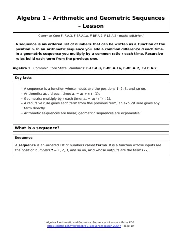
A sequence is an ordered list of numbers that can be written as a function of the position n. In an arithmetic sequence you add a common difference d each time. In a geometric sequence you multiply by a common ratio r each time. Recursive rules build each term from the previous one.

Algebra 1 · Common Core State Standards: F-IF.A.3, F-BF.A.1a, F-BF.A.2, F-LE.A.2

Key facts in this sequences lesson

What is a sequence?

What is an arithmetic sequence?

In an arithmetic sequence, you add the same number, the common difference \(d\), to get the next term.

The recursive rule says how to get a term from the previous one: \(a_{n} = a_{n-1} + d\). The explicit rule gives any term directly: \(a_{n} = a_{1} + (n – 1)d\). For 4, 7, 10, 13 this is \(a_{n} = 4 + (n – 1)(3)\), which simplifies to \(a_{n} = 3n + 1\).

What is a geometric sequence?

In a geometric sequence, you multiply by the same number, the common ratio \(r\), each time.

The recursive rule is \(a_{n} = r \cdot a_{n-1}\) and the explicit rule is \(a_{n} = a_{1} \cdot r^{n-1}\). For 3, 6, 12, 24 the explicit rule is \(a_{n} = 3 \cdot 2^{n-1}\), so the 8th term is \(3 \cdot 2^{7} = 384\).

How do you write a rule for a sequence?

1. Subtract consecutive terms. If the differences match, it is arithmetic.
2. Divide consecutive terms. If the ratios match, it is geometric.
3. Substitute the first term and the common difference or ratio into the explicit rule.
4. Check the rule with the first two terms.

Example: The figures use 5, 7, and 9 squares. The differences are 2, so the rule is \(a_{n} = 5 + (n – 1)(2)\), which simplifies to \(a_{n} = 2n + 3\). Figure 10 uses \(2(10) + 3 = 23\) squares.

Arithmetic sequences grow by equal steps, so they are linear. Geometric sequences grow by equal factors, so they are exponential.

Tip: Check a rule with the first two terms before you use it. For \(a_{n} = 3n + 1\), the first term is \(3(1) + 1 = 4\) and the second is \(3(2) + 1 = 7\), which match the list.

Sequences lesson: questions and answers

How to use this sequences lesson

Read the definitions first, then follow the worked method line by line and redo the example on paper without looking. When every step makes sense, move on to the worksheet, then check yourself with the quiz.

Download the sequences lesson as a PDF with the button below and keep it with your notes.

All Algebra 1 chapters: Algebra 1 math.